Spiking neural networks: teaching a model to think in spikes
I built a leaky integrate-and-fire spiking network in snnTorch that reaches 98% on MNIST using discrete spikes over time instead of continuous activations. Here is how event-driven inference actually works, and why it matters for edge hardware.
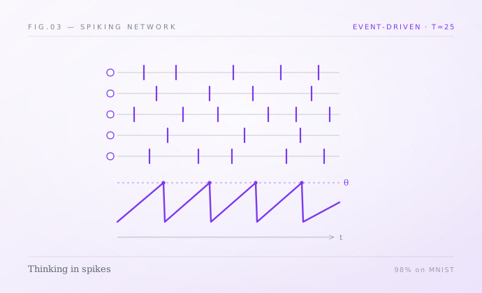
A standard network answers in a single shot. A spiking network answers by accumulating evidence over time, the way a real neuron does.
Almost every model I build passes around continuous numbers: a pixel is 0.73, a hidden unit fires 1.84, a logit is -0.5. Real neurons do not work like that. They sit quietly until enough charge builds up, fire a brief electrical spike, reset, and start again. The information is not in the size of a number. It is in when and how often a neuron spikes.
Spiking neural networks (SNNs), sometimes called the "third generation" of neural networks, take that idea literally. I wanted to actually build one rather than just read about them, so I trained a small SNN on MNIST in snnTorch and PyTorch. It reaches 98% test accuracy, within about a point of an equivalent dense network, but it gets there in a completely different way. The full notebook is on GitHub at vnimesha/SNN.
The neuron is a leaky bucket
The building block is a leaky integrate-and-fire (LIF) neuron. Picture a bucket with a small hole in the bottom:
- Incoming spikes pour charge in, raising the membrane potential
V. - The hole leaks charge away over time, controlled by a decay factor
β(here0.9). - When
Vcrosses a threshold, the neuron emits a spike and resets.
Each timestep, the update is essentially:
V(t+1) = β · V(t) + (weighted input spikes) − (threshold if it just fired)With β = 0.9, the neuron keeps 90% of its charge between steps, so it has a short memory: recent inputs matter more than old ones. That single stateful equation is what makes an SNN fundamentally temporal. There is no single forward pass; there is a little simulation running inside every neuron.
Turning a static image into spikes
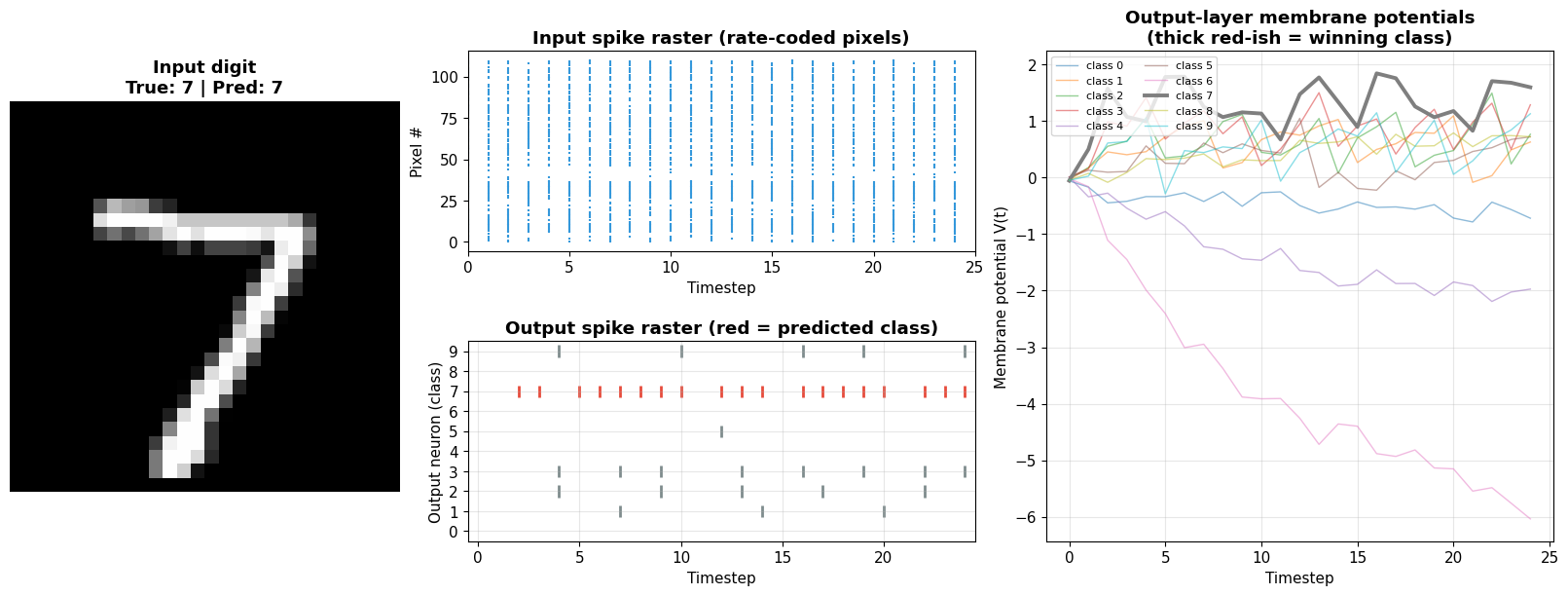
MNIST images are static, so before the network can process one I have to convert it into spike trains. I use rate coding: a brighter pixel spikes more often. A pixel with intensity 0.8 fires a spike with 80% probability on each of T = 25 timesteps, producing a stochastic stream of 0s and 1s.
# rate coding: pixel intensities become spike trains over T timesteps
# (batch, 1, 28, 28) -> (T, batch, 1, 28, 28)
spike_input = spikegen.rate(x, num_steps=NUM_TIMESTEPS)
spike_input = spike_input.view(NUM_TIMESTEPS, x.size(0), -1)
So a single digit becomes 25 noisy binary frames. The network never sees the smooth grayscale image; it sees a flicker of spikes and has to integrate them into a decision.
The network
Architecturally it looks ordinary: three linear layers, 784 → 256 → 128 → 10, about 235K parameters. The twist is that every linear layer feeds a LIF neuron instead of a ReLU, and the whole thing is unrolled over time.
class SpikingNet(nn.Module):
    def __init__(self):
        super().__init__()
        self.fc1 = nn.Linear(28 * 28, 256)
        self.fc2 = nn.Linear(256, 128)
        self.fc3 = nn.Linear(128, NUM_CLASSES)
        # one LIF neuron per layer; snn.Leaky handles the membrane
        # update, threshold check, spike, and reset internally
        self.lif1 = snn.Leaky(beta=BETA)
        self.lif2 = snn.Leaky(beta=BETA)
        self.lif3 = snn.Leaky(beta=BETA)

    def forward(self, x):
        spike_input = spikegen.rate(x, num_steps=NUM_TIMESTEPS)
        spike_input = spike_input.view(NUM_TIMESTEPS, x.size(0), -1)

        mem1, mem2, mem3 = self.lif1.init_leaky(), self.lif2.init_leaky(), self.lif3.init_leaky()
        spike_record, mem_record = [], []

        for t in range(NUM_TIMESTEPS):              # simulate the network in time
            cur1 = self.fc1(spike_input[t])
            spk1, mem1 = self.lif1(cur1, mem1)
            cur2 = self.fc2(spk1)
            spk2, mem2 = self.lif2(cur2, mem2)
            cur3 = self.fc3(spk2)
            spk3, mem3 = self.lif3(cur3, mem3)
            spike_record.append(spk3)
            mem_record.append(mem3)

        return torch.stack(spike_record), torch.stack(mem_record)
Notice the for t in range(NUM_TIMESTEPS) loop. The same weights are applied 25 times, and the membrane potentials mem1/2/3 carry state forward between steps. The output is not a vector of logits; it is a record of which output neurons spiked, at every timestep.
To classify, I simply count spikes. The output neuron that fires the most over the 25 steps wins.
The hard part: you cannot differentiate a spike
Here is the problem that makes SNNs interesting to train. A spike is a step function: the neuron outputs 0, then suddenly 1. The derivative of that step is zero almost everywhere and undefined at the threshold. Backpropagation needs a gradient, and a spike does not give you a useful one.
The trick is the surrogate gradient. On the forward pass the neuron fires a hard binary spike, but on the backward pass we pretend the spike was a smooth, differentiable curve (a fast sigmoid) so gradients can flow. snnTorch applies this automatically and unrolls the loss backward through all 25 timesteps, which is backpropagation through time. The loss itself is cross-entropy on the per-class spike counts.
optimizer = torch.optim.Adam(model.parameters(), lr=1e-3)
loss_fn = SF.ce_count_loss()                 # cross-entropy on spike counts

for images, labels in train_loader:
    spike_record, _ = model(images)          # simulate over T steps
    loss = loss_fn(spike_record, labels)
    optimizer.zero_grad()
    loss.backward()                          # surrogate gradients, applied through time
    optimizer.step()
That is the whole training story: forward in spikes, backward in surrogates, optimize the counts.
Results
After 15 epochs the network reaches 98.0% test accuracy (99.5% on train). For a from-scratch spiking model on raw rate-coded input, landing within about a point of a conventional dense network is a satisfying result.
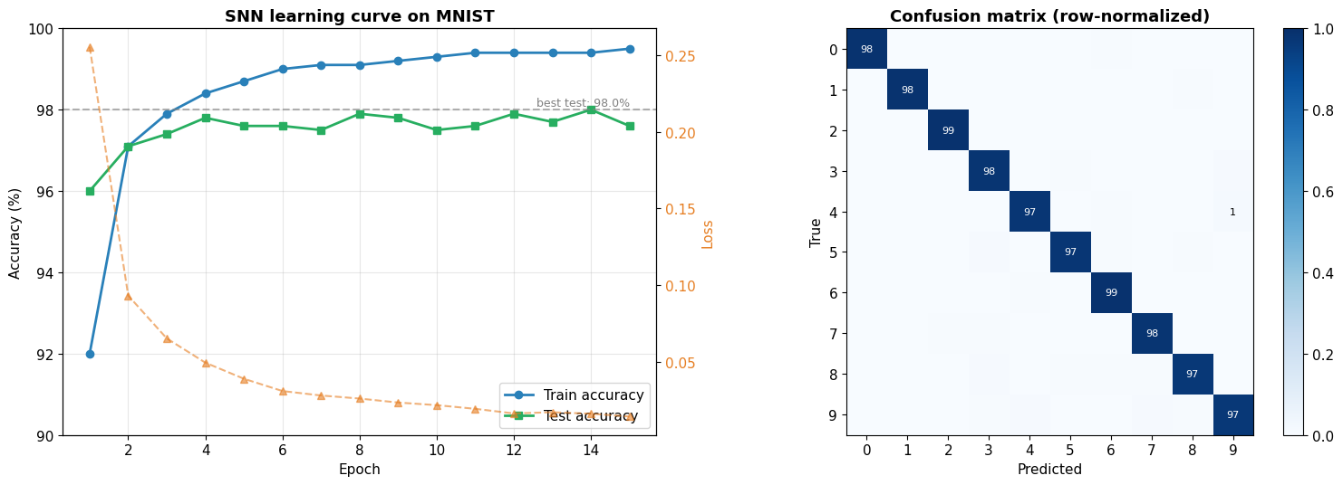
The predictions look like any other MNIST classifier from the outside, but remember that each call to the network is a 25-step simulation, not a single matrix multiply.

The most interesting plot is the internal dynamics. If you watch the output membrane potentials over time, you can see the network make up its mind: the correct class climbs steadily while the others stay flat. Classification is a race, and the fastest-rising neuron wins.
SNN vs ANN, side by side
| Aspect | Standard ANN | Spiking network |
|---|---|---|
| Signal | Continuous floats | Binary spikes (0/1) over time |
| Time | Single forward pass | Simulated over T timesteps |
| Neuron | ReLU / GELU | LIF (stateful, leaky integrator) |
| Computation | Dense multiply-accumulate | Event-driven and sparse |
| Hardware fit | GPU / TPU | Neuromorphic chips |
| Energy | High, constant | Potentially 10 to 100x lower |
| Training | Direct backprop | Surrogate gradients through time |
Why I cared enough to build this
My day job involves squeezing vision models onto edge hardware, where the budget is milliwatts, not watts. SNNs are the extreme end of that idea: because computation only happens when a neuron actually spikes, the work is sparse, and neuromorphic chips (Intel Loihi 2, BrainChip Akida) exploit that for very low power, always-on inference. Building one by hand was the fastest way to understand what that hardware is really doing.
What I took away
Three things stuck with me. First, time is a feature, not a nuisance: giving the model a temporal axis to integrate evidence over is a genuinely different computational style, and it is a natural fit for event-camera and audio data that is already temporal. Second, non-differentiable does not mean untrainable: the surrogate-gradient trick is a clean, general idea for pushing gradients through hard decisions. Third, accuracy is only one axis: an SNN that matches an ANN on MNIST while opening the door to 10 to 100x lower energy is winning on a metric the accuracy number alone never shows.
If you want to poke at the dynamics yourself, the notebook (architecture, training, and all the visualizations) is at vnimesha/SNN. It runs in about five minutes on a GPU.
Vihanga Nimesha
Software & AI engineer building things that ship. More about me